2D Robot Arm Inverse Kinematics using Mixed Integer Programming in Cvxpy
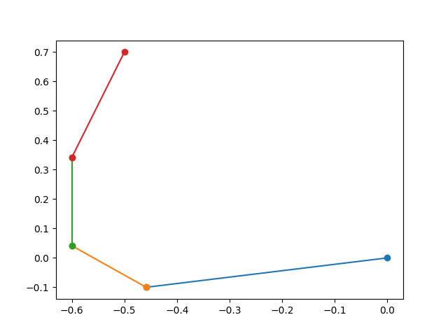
Mixed Integer programming is crazy powerful. You can with ingenuity encode many problems into it. The following is a simplification of the ideas appearing in http://groups.csail.mit.edu/robotics-center/public_papers/Dai19.pdf . They do 3d robot arms, I do 2d. I also stick to completely linear approximations.
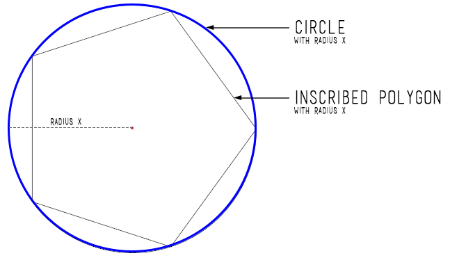
The surface of a circle is not a convex shape. If you include the interior of a circle it is. You can build a good approximation to the circle as polygons. A polygon is the union of it’s sides, each of which is a line segment. Line sgements are convex set. Unions of convex sets are encodable using mixed integer programming. What I do is sample N regular positions on the surface of a circle. These are the vertices of my polygon. Then I build boolean indicator variables for which segment we are on. Only one of them is be nonzero $ \sum s_i == 1$. If we are on a segment, we are allowed to make positions $ x$ that interpolate between the endpoints $ x_i$ of that segment $ x = \lambda_1 x_1 + \lambda_2 x_2$, where $ \lambda_i >= 0$ and $ \sum \lambda=1$. These $ \lambda$ are only allowed to be nonzero if we are on the segment, so we suppress them with the indicator variables $ \lambda_i <= s_i + s_{i+1}$. That’s the gist of it.
Given a point on the circle (basically sines and cosines of an angle) we can build a 2d rotation matrix $ R$ from it. Then we can write down the equations connecting subsequent links on the arm. $ p_{i+1}=p_{i} +Rl$. By using global rotations with respect to the world frame, these equations stay linear. That is a subtle point. $ p$ and $ R$ are variables, whereas $ l$ is a constant describing the geometry of the robot arm. If we instead used rotation matrices connecting frame i to i+1 these R matrices would compound nonlinearly.
All in all, pretty cool!
import cvxpy as cvx
import numpy as np
import matplotlib.pyplot as plt


# builds a N sided polygon approximation of a circle for MIP. It is the union of the segments making up the polygon
# might also be useful to directly encode arcs. for joint constraint limits.
def circle(N):
    x = cvx.Variable()
    y = cvx.Variable()
    l = cvx.Variable(N) #interpolation variables
    segment = cvx.Variable(N,boolean=True) #segment indicator variables, relaxing the boolean constraint gives the convex hull of the polygon

    angles = np.linspace(0, 2*np.pi, N, endpoint=False)
    xs = np.cos(angles) #we're using a VRep
    ys = np.sin(angles)

    constraints = []
    constraints += [x == l*xs, y == l*ys] # x and y are convex sum of the corner points
    constraints += [cvx.sum(l) == 1, l <= 1, 0 <= l] #interpolations variables. Between 0 and 1 and sum up to 1
    constraints += [cvx.sum(segment) == 1] # only one indicator variable can be nonzero

    constraints += [l[N-1] <= segment[N-1] + segment[0]] #special wrap around case
    for i in range(N-1):
        constraints += [l[i] <= segment[i] + segment[i+1]] # interpolation variables suppressed
    return x, y, constraints

x, y, constraints = circle(8)
objective = cvx.Maximize(x-0.8*y)
prob = cvx.Problem(objective, constraints)
res = prob.solve(solver=cvx.GLPK_MI, verbose=True)

# build a 2d rotation matrix using circle
def R(N):
    constraints = []
    c, s, constraint = circle(N) # get cosines and sines from a circle
    constraints += constraint

    r = cvx.Variable((2,2)) # build rotation matrix
    constraints += [r[0,0] == c, r[0,1] == s]
    constraints += [r[1,0] == -s, r[1,1] == c]
    return r, constraints
    # np.array([[c , s],                [-s, c]])

#robot linkage of differing arm length
link_lengths = [0.5,0.2,0.3,0.4]
pivots = []
Rs = []
N = 8
constraints = []
origin = np.zeros(2)

p1 = origin
for l in link_lengths:
    R1, c = R(8)
    constraints += c

    p2 = cvx.Variable(2)
    constraints += [p2 == p1 + R1*np.array([l,0])] # R1 is global rotation with respect to world frame. This is important. It is what makes the encoding linear.

    p1 = p2

    pivots.append(p2)
    Rs.append(R1)

end_position = np.array([-0.5, .7])
constraints += [p2 == end_position]

objective = cvx.Maximize(1)
prob = cvx.Problem(objective, constraints)
res = prob.solve(solver=cvx.GLPK_MI, verbose=True)
print(res)

#print(R(x,y))

print(p2.value)
print(list(map(lambda r: r.value, Rs)))
#print(y.value)

p1 = origin
for l, r in zip(link_lengths, Rs):
    p2 = p1 + r.value@np.array([l,0])
    plt.plot([p1[0],p2[0]], [p1[1],p2[1]], marker='o'),

    p1 = p2
plt.show()

'''
print(xs)
print(ys)
print(angles)

print(l.value)
print(segment.value)
plt.plot(x.value, label='x')
plt.plot(v.value, label= 'v')
plt.plot(collision.value, label = 'collision bool')
plt.legend()
plt.xlabel('time')
plt.show()
'''

