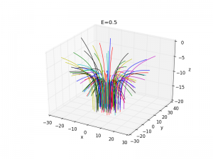
A fun little man of rutherford scattering

So I coded up rutherford scattering in a real dumb way (you can significantly reduce your considerations by using symmetry and stuff).

I sort of monte carlo it with gaussian distributed initial conditions

import numpy as np
from scipy import integrate

z0 = -20.0
samples = 100
E=.5
t = np.linspace(0,50,100)


def F(x):
    return .1 * x / np.linalg.norm(x)**1.5

def D(x,t):
    return np.concatenate((x[3:],F(x[0:3])))



import matplotlib.pyplot as plt
from mpl_toolkits.mplot3d import Axes3D
fig = plt.figure()
ax = fig.add_subplot(111, projection='3d')
ax.set_xlabel('x')
ax.set_ylabel('y')
ax.set_zlabel('z')



def update(E):
    ax.set_title('E='+str(E))
    for i in range(samples):
        initxy = 5*np.random.randn(2)
        init = np.append(initxy,[z0, 0., 0., np.sqrt(E)])
        sol = integrate.odeint(D, init, t)
        ax.plot(sol[:,0], sol[:,1],sol[:,2])
update(E)

plt.show()

The bundles that come off look pretty cool

Lots that one could do with this. Compare the outgoing distribution to the formula, Try to discern shape of other potentials. Do a little statistics to see if charge or whatever can be determined from the data.

Show center of mass scattering. Try 4 particle scattering.

I guess I’m trying to play around in some high energy concepts.