Cart Pole Trajectory optimization using Cvxpy
I’ve been watching Russ Tedrake’s underactuated robotics and been trying some stuff out. The Drake package probably does this stuff better. Also IpOpt and Snopt are the libraries that get mentioned when people want to do this stuff for real.
It’s too slow to be practical. That is mostly the fault of the cvxpy overhead. The ECOS solver itself says that it solves each iteration in about 0.02 seconds on my macbook.
The idea is to use linearized dynamics as constraints. Then iteratively ask cvxpy to solve for us. Until hopefully it converges. This is Sequential Convex Programming https://web.stanford.edu/class/ee364b/lectures/seq_slides.pdf
I used the discretization of the equations of motion using the mehotd described here https://epubs.siam.org/doi/pdf/10.1137/16M1062569
It is possible I did it right.
The Hermite Collocation for the trajectory and trapezoidal for the control
If we used just an absolute value cost, this all would be a linear program. Something to consider. Also CVXOPT would probably be faster.
It hurts me that the constraint and cost matrices are banded and could be solved so quickly. But the next level up in programming complexity takes a lot more work it seems to me.
import numpy as np
import scipy as sp
import cvxpy as cvx
import matplotlib.pyplot as plt

g = 9.8
l = 1.0
dt = 0.1
lookahead = 100


def f(x, u):
    #print(x)
    b = np.zeros_like(x)
    theta = x[0]
    dtheta = x[1]
    a = u[0]
    b[0] = dtheta
    b[1] = (a * np.cos(theta) - g * np.sin(theta)) / l
    return b

def df(x, u):
    A = np.zeros((x.shape[0], x.shape[0]))
    B = np.zeros((x.shape[0], u.shape[0]))
    theta = x[0]
    dtheta = x[1]
    a = u[0]
    # dthetadot / dtheta
    A[0,1] = 1
    # dtheta derviatvie.
    A[1,0] = (- a * np.sin(theta) - g * np.cos(theta)) / l
    B[1,0] = np.cos(theta) / l
    #b[1,:] = (a * np.cos(theta) - g * np.sin(theta)) / l
    return A, B

def linf(x, u, x2, u2):
    b = f(x,u)
    A, B = df(x,u)
    return b + A @ (x2 - x) + B * (u2 - u)


np_x = np.zeros((2*lookahead+1, 2))

np_u = np.zeros((lookahead+1, 1))
for j in range(15):
    controls = []
    constraints = []
    thetas = []
    dthetas = []
    xs = []
    cost = 0


    #initiial condition constraints

    x = cvx.Variable(2)
    constraints.append(x[0] == 0)
    constraints.append(x[1] == 0)


    xs.append(x)

    u = cvx.Variable(1)
    constraints.append(u <= 13.0)
    constraints.append(u >= -13.0)
    controls.append(u)

    for i in range(lookahead):
        next_u = cvx.Variable(1)
        controls.append(next_u)

        # next time step variables
        next_x = cvx.Variable(2)
        half_x = cvx.Variable(2)

        #delthetan = cvx.Variable()
        #deldthetan = cvx.Variable()
        #delthetas.append(delthetan)
        #deldthetas.append(deldthetan)
        xs.append(half_x)
        xs.append(next_x)
        #lin = linearApproxAlpha(a[i], theta[i])

        #Dynamics

        constraints.append(half_x == next_x/2 + x/2 + dt/8 * (linf(np_x[2*i,:], np_u[i,:],x, u ) - linf(np_x[2*i+2,:], np_u[i+1,:],next_x, next_u )))

        constraints.append(next_x - x ==  (linf(np_x[2*i,:], np_u[i,:], x, u ) + 4 * linf(np_x[2*i+1,:], (np_u[i,:] + np_u[i+1,:]) / 2, half_x, (u + next_u)/2) + linf(np_x[2*i+2,:], np_u[i+1,:], next_x, next_u )  ) * dt / 6)
        #constraints.append(deldthetan == deldtheta + lin(at, deltheta) * dt)

        #conditions on allowable control
        constraints.append(next_u <= 8.0)
        constraints.append(next_u >= -8.0)
        #trust regions


        #Cost calculation
        cost = cost + cvx.huber( x[0] - np.pi, M=0.5) + 0.01 * cvx.huber(u)#+ (np.cos(np_x[2*i,:]) + 1) * (x[0] - np_x[2*i,:])  #+ cvx.square( x[0] - np.pi ) #+ cvx.square(u) #+ 0.1 * cvx.square(ut)
        # + cvx.square(np.cos(np_x[2*i,:])*(x - np_x[2*i,:]))
        x = next_x
        u = next_u


    cost = cost + 100 * cvx.square( x[0] - np.pi )  # cvx.huber( x[0] - np.pi, M=0.4)
    objective = cvx.Minimize(cost)
    #print(objective)
    #print(constraints)
    prob = cvx.Problem(objective, constraints)
    sol = prob.solve(verbose=True)
    #print(sol)
    #update by the del
    #theta += np.array(list(map( lambda x: x.value, delthetas)))
    #print(x.value)
    #print(constraints[0])
    np_x = np.array(list(map( lambda x: x.value, xs)))
    print(np_x.shape)
    np_x = np_x.reshape((-1,2))
    print(np_x.shape)
    np_u = np.array(list(map( lambda x: x.value, controls))).reshape((-1,1))
    '''
    plt.plot(np_x[::2,0])
    plt.plot(np_x[::2,1])
    plt.plot(np_u[:,0])

    plt.show()
    '''
    #dtheta += np.array(list(map( lambda x: x.value, deldthetas)))
    #a += np.array(list(map( lambda x: x.value, controls)))

#print(np_u)

plt.plot(np_x[::2,0])
plt.plot(np_x[::2,1])
plt.plot(np_u[:,0])

plt.show()


#TODO
'''
We need to add cart position contraints
Parameters to hopefully speed up
Better initial guess.
Derivative of Cost
Is this actually working?
'''
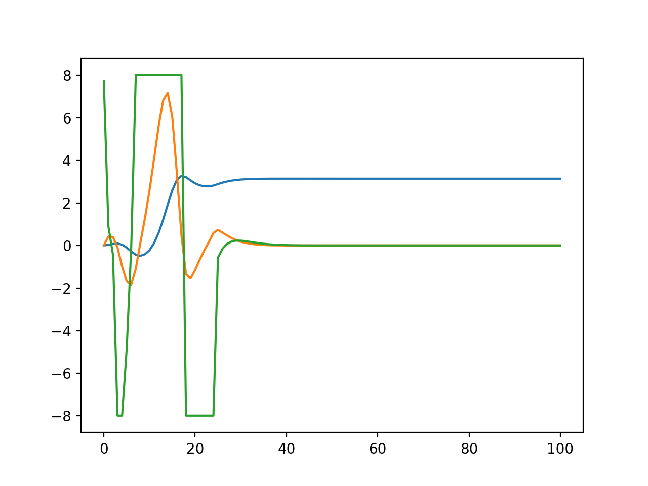
This is the result
Green is cart acceleration. You can see it slamming into the maximum acceleration constraint
Blue is pole angle and orange is angular velocity. So it does a pretty good job. For some settings it is just awful though.
