Deriving the Chebyshev Polynomials using Sum of Squares optimization with Sympy and Cvxpy
Least squares fitting $ \sum (f(x_i)-y_i)^2$ is very commonly used and well loved. Sum of squared fitting can be solved using just linear algebra. One of the most convincing use cases to me of linear programming is doing sum of absolute value fits $ \sum |f(x_i)-y_i|$ and maximum deviation fits $ \max_i |f(x_i)-y_i|$. These two quality of fits are basically just as tractable as least squares, which is pretty cool.
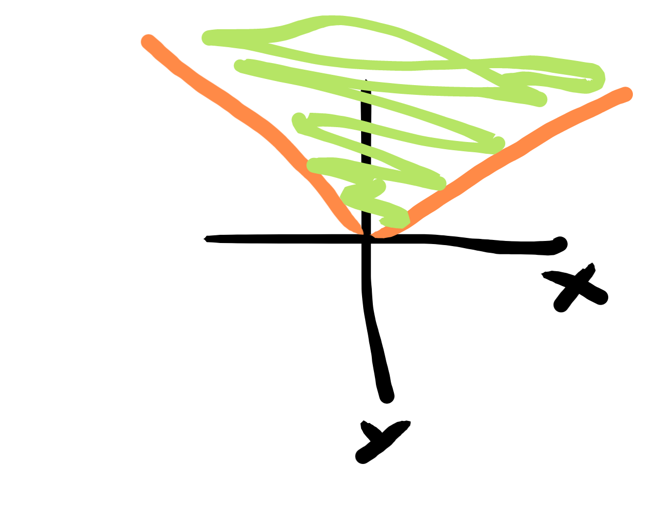
The trick to turning an absolute value into an LP is to look at the region above the graph of absolute value.
This region is defined by $ y \ge x$ and $ y \ge -x$. So you introduce a new variable y. Then the LP $ \min y$ subject to those constraints will minimize the absolute value. For a sum of absolute values, introduce a variable $ y_i$ for each absolute value you have. Then minimize $ \sum_i y_i$. If you want to do min max optimization, use the same y value for every absolute value function.
$ \min y$
$ \forall i. -y \le x_i \le y$
Let’s change topic a bit. Chebyshev polynomials are awesome. They are basically the polynomials you want to use in numerics.
Chebyshev polynomials are sines and cosines in disguise. They inherit tons of properties from them. One very important property is the equioscillation property. The Chebyshev polynomials are the polynomials that stay closest to zero while keeping the x^n coefficient nonzero (2^(n-2) by convention). They oscillate perfectly between -1 and 1 on the interval $ x \in [-1,1]$ just like sort of a stretched out sine. It turns out this equioscillation property defines the Chebyshev polynomials
We can approximate the Chebyshev polynomials via sampling many points between [-1,1]. Then we do min of the max absolute error optimization using linear programming. What we get out does approximate the Chebyshev polynomials.
import cvxpy as cvx
import numpy as np
import matplotlib.pyplot as plt

# try finding the 3 through 5 chebyshev polynomial
for N in range(3,6):
	a = cvx.Variable(N) #polynomial coefficients
	t = cvx.Variable()
	n = np.arange(N) #exponents


	xs = np.linspace(-1,1,100)
	chebcoeff = np.zeros(N)
	chebcoeff[-1] = 1
	plt.plot(xs, np.polynomial.chebyshev.chebval(xs, chebcoeff), color='r')

	constraints = [a[-1]==2**(N-2)] # have to have highest power
	for k in range(100):
	   x = np.random.rand()*2-1 #pick random x in [-1,1]
	   c = cvx.sum(a * x**n) #evaluate polynomial

	   constraints.append(c <= t)
	   constraints.append(-t <= c)

	obj = cvx.Minimize(t) #minimize maximum aboslute value
	prob = cvx.Problem(obj,constraints)
	prob.solve()
	plt.plot(xs, np.polynomial.polynomial.polyval(xs, a.value), color='g')
	print(a.value)

plt.show()
Found Coefficients:
[-9.95353054e-01  1.33115281e-03  1.99999613e+00]
[-0.01601964 -2.83172979  0.05364805  4.00000197]
[ 0.86388003 -0.33517716 -7.4286604   0.6983382   8.00000211]
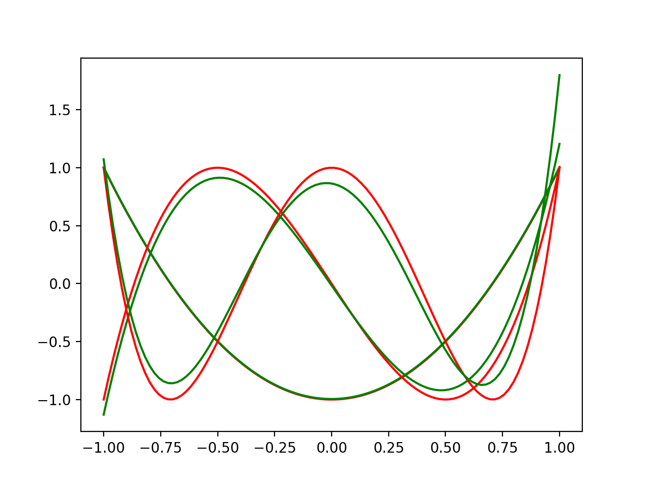
Red is the actual Chebyshev polynomials and green is the solved for polynomials. It does a decent job. More samples will do even better, and if we picked the Chebyshev points it would be perfect.
Can we do better? Yes we can. Let’s go on a little optimization journey.
Semidefinite programming allows you to optimize matrix variables with the constraint that they have all positive eigenvalues. In a way it lets you add an infinite number of linear constraints. Another way of stating the eigenvalue constraint is that
$ \forall q. q^T X q \ge 0$
You could sample a finite number of random q vectors and take the conjunction of all these constraints. Once you had enough, this is probably a pretty good approximation of the Semidefinite constraint. But semidefinite programming let’s you have an infinite number of the constraints in the sense that $ \forall q$ is referencing an infinite number of possible q , which is pretty remarkable.
Finite Sampling the qs has similarity to the previously discussed sampling method for absolute value minimization.
Sum of Squares optimization allows you to pick optimal polynomials with the constraint that they can be written as a sum of squares polynomials. In this form, the polynomials are manifestly positive everywhere. Sum of Squares programming is a perspective to take on Semidefinite programming. They are equivalent in power. You solve SOS programs under the hood by transforming them into semidefinite ones.
You can write a polynomial as a vector of coefficients $ \tilde{a}$.
$ \tilde{x} = \begin{bmatrix} 1 \ x \ x^2 \ x^3 \ \vdots \end{bmatrix}$
$ \tilde{a} = \begin{bmatrix} a_0 \ a_1 \ a_2 \ a_3 \ \vdots \end{bmatrix}$
$ p(x)=\tilde{a}^T \tilde{x}$
Instead we represent the polynomial with the matrix $ Q$
$ p(x) = \tilde{x}^T Q \tilde{x}$
If the matrix is positive semidefinite, then it can be diagonalized into the sum of squares form.
In all honesty, this all sounds quite esoteric, and it kind of is. I struggle to find problems to solve with this stuff. But here we are! We’ve got one! We’re gonna find the Chebyshev polynomials exactly by translating the previous method to SOS.
The formulation is a direct transcription of the above tricks.
$ \min t$
$ -t \le p(x) \le t$ by which I mean $ p(x) + t$ is SOS and $ t - p(x)$ is SOS.
There are a couple packages available for python already that already do SOS, .
ncpol2sdpa (https://ncpol2sdpa.readthedocs.io/en/stable/)
Irene (https://irene.readthedocs.io/en/latest/index.html)
SumofSquares.jl for Julia and SOSTools for Matlab. YalMip too I think. Instead of using those packages, I want to roll my own, like a doofus.
Sympy already has very useful polynomial manipulation functionality. What we’re going to do is form up the appropriate expressions by collecting powers of x, and then turn them into cvxpy expressions term by term. The transcription from sympy to cvxpy isn’t so bad, especially with a couple helper functions.
One annoying extra thing we have to do is known as the S-procedure. We don’t care about regions outside of $ x \in [-1,1]$. We can specify this with a polynomial inequality $ (x+1)(x-1) \ge 0$. If we multiply this polynomial by any manifestly positive polynomial (a SOS polynomial in particular will work), it will remain positive in the region we care about. We can then add this function into all of our SOS inequalities to make them easier to satisfy. This is very similar to a Lagrange multiplier procedure.
Now all of this seems reasonable. But it is not clear to me that we have the truly best polynomial in hand with this s-procedure business. But it seems to works out.
from sympy import *
import cvxpy as cvx
import matplotlib.pyplot as plt
import numpy as np

#build corresponding cvx variable for sympy variable
def cvxvar(expr, PSD=True):
    if expr.func == MatrixSymbol:
        i = int(expr.shape[0].evalf())
        j = int(expr.shape[1].evalf())
        return cvx.Variable((i,j), PSD=PSD)
    elif expr.func == Symbol:
        return cvx.Variable()

def cvxify(expr, cvxdict): # replaces sympy variables with cvx variables
     return lambdify(tuple(cvxdict.keys()), expr)(*cvxdict.values())


xs = np.linspace(-1,1,100)

for N in range(3,6):
    #plot actual chebyshev
    chebcoeff = np.zeros(N)
    chebcoeff[-1] = 1
    plt.plot(xs, np.polynomial.chebyshev.chebval(xs, chebcoeff), color='r')

    cvxdict = {}
    # Going to need symbolic polynomials in x
    x = Symbol('x')
    xn = Matrix([x**n for n in range(N)]);

    def sospoly(varname):
        Q = MatrixSymbol(varname, N,N)
        p = (xn.T * Matrix(Q) * xn)[0]
        return p, Q

    t = Symbol('t')
    cvxdict[t] = cvxvar(t)

    #lagrange multiplier polynomial 1
    pl1, l1 = sospoly('l1')
    cvxdict[l1] = cvxvar(l1)

    #lagrange multiplier polynomial 2
    pl2, l2 = sospoly('l2')
    cvxdict[l2] = cvxvar(l2)

    #Equation SOS Polynomial 1
    peq1, eq1 = sospoly('eq1')
    cvxdict[eq1] = cvxvar(eq1)

    #Equation SOS Polynomial 2
    peq2, eq2 = sospoly('eq2')
    cvxdict[eq2] = cvxvar(eq2)

    a = MatrixSymbol("a", N,1)
    pa = Matrix(a).T*xn #sum([polcoeff[k] * x**k for k in range(n)]);
    pa = pa[0]
    cvxdict[a] = cvxvar(a, PSD=False)


    constraints = []


    # Rough Derivation for upper constraint
    # pol <= t
    # 0 <= t - pol + lam * (x+1)(x-1)  # relax constraint with lambda
    # eq1 = t - pol + lam
    # 0 = t - pol + lam - eq1
    z1 = t - pa + pl1 * (x+1)*(x-1) - peq1
    z1 = Poly(z1, x).all_coeffs()
    constraints += [cvxify(expr, cvxdict) == 0 for expr in z1]

    # Derivation for lower constraint
    # -t <= pol
    # 0 <= pol + t + lam * (x+1)(x-1) # relax constraint with lambda
    # eq2 = pol + t + lam     # eq2 is SOS
    # 0 = t - pol + lam - eq2     #Rearrange to equal zero.
    z2 = pa + t + pl2 * (x+1)*(x-1) - peq2
    z2 = Poly(z2, x).all_coeffs()
    constraints += [cvxify(expr, cvxdict) == 0 for expr in z2]

    constraints += [cvxdict[a][N-1,0] == 2**(N-2) ]
    obj = cvx.Minimize(cvxdict[t]) #minimize maximum absolute value
    prob = cvx.Problem(obj,constraints)
    prob.solve()

    print(cvxdict[a].value.flatten())
    plt.plot(xs, np.polynomial.polynomial.polyval(xs, cvxdict[a].value.flatten()), color='g')


plt.show()


Coefficients:
[-1.00000000e+00 -1.02219773e-15  2.00000001e+00]
[-1.23103133e-13 -2.99999967e+00  1.97810058e-13  4.00001268e+00]
[ 1.00000088e+00 -1.39748880e-15 -7.99999704e+00 -3.96420452e-15
  7.99999691e+00]
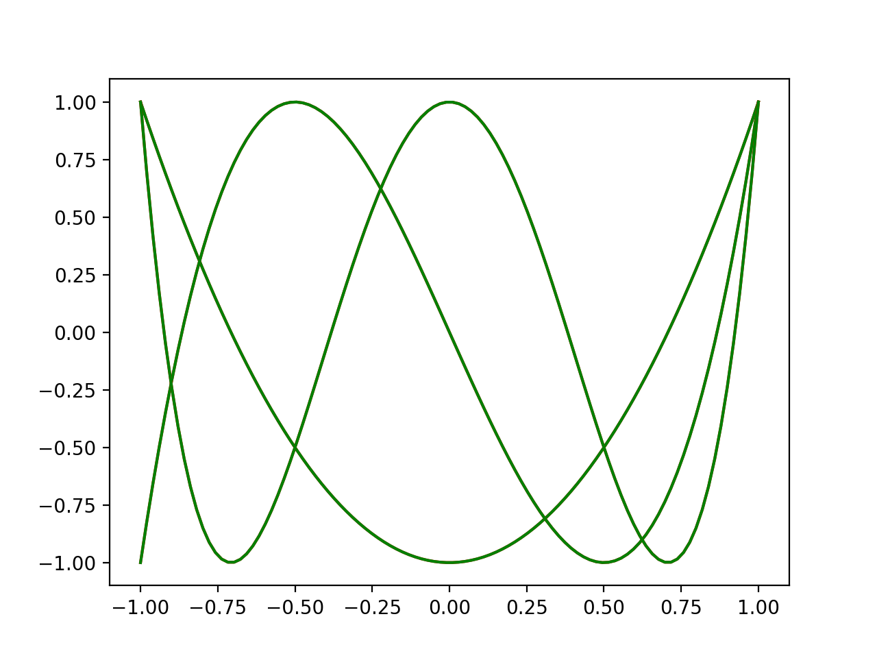
Ooooooh yeah. Those curves are so similar you can’t even see the difference. NICE. JUICY.
There are a couple interesting extension to this. We could find global under or over approximating polynomials. This might be nice for a verified compression of a big polynomial to smaller, simpler polynomials for example. We could also similar form the pointwise best approximation of any arbitrary polynomial f(x) rather than the constant 0 like we did above (replace $ -t \le p(x) \le t$ for $ -t \le p(x) - f(x) \le t$ in the above). Or perhaps we could use it to find a best polynomial fit for some differential equation according to a pointwise error.
I think we could also extend this method to minimizing the mean absolute value integral just like we did in the sampling case.
$ \min \int_0^1 t(x)dx$
$ -t(x) \le p(x) \le t(x)$
More references on Sum of Squares optimization:
https://www.youtube.com/watch?v=HdZajqWl15I
https://www.youtube.com/watch?v=GSneSgtellY


