Extracting a Banded Hessian in PyTorch
So pytorch does have some capability towards higher derivatives, with the caveat that you have to dot the gradients to turn them back into scalars before continuing. What this means is that you can sample a single application of the Hessian (the matrix of second derivatives) at a time.
One could sample out every column of the hessian for example. Performance-wise I don’t know how bad this might be.
For a banded hessian, which will occur in a trajectory optimization problem (the bandedness being a reflection of the finite difference scheme), you don’t need that many samples. This feels more palatable. You only need to sample the hessian roughly the bandwidth number of times, which may be quite small. Plus, then you can invert that banded hessian very quickly using special purpose banded matrix solvers, which are also quite fast. I’m hoping that once I plug this into the trajectory optimization, I can use a Newton method (or SQP?) which will perform better than straight gradient descent.
If you pulled just a single column using [1,0,0,0,0,0..] for example, that would be wasteful, since there are so many known zeros in the banded matrix. Instead something like [1,0,0,1,0,0,1,0,0..] will not have any zeros in the result. This gets us every 3rd row of the matrix. Then we can sample with shifted versions like [0,1,0,0,1,0,0,1,0,0..]. until we have all the rows somewhere. Then there is some index shuffling to put the thing into a sane ordering, especially so that we can use https://docs.scipy.org/doc/scipy/reference/generated/scipy.linalg.solveh_banded.html which requires the banded matrix to be given in a particular form.
An alternative approach might be to use an fft with some phase twiddling. Also it feels like since the Hessian is hermitian we ought to be able to use about half the samples, since half are redundant, but I haven’t figured out a clean way to do this yet. I think that perhaps sampling with random vectors and then solving for the coefficients would work, but again how to organize the code for such a thing?
Here’s a snippet simulatng extracting the band matrix from matrix products.
import numpy as np

N = 6
B = 5
h = np.diag(np.random.randn(N))
h = h + h.T # symmetrize our matrix
print(h)
band = y = np.zeros((B, N))
for i in range(B):
	y = np.zeros(N)
	y[i::B]=1
	band[i,:] = h @ y
print(band)
for i in range(B):
	band[:,i::B] = np.roll(band[:,i::B], -i, axis=0) #B//2

print(band)
print(band[:B//2+1,:])
and here is the full pytorch implementation including a linear banded solve.
import torch
import matplotlib.pyplot as plt
import numpy as np
import torch.optim
from scipy import linalg
import matplotlib.pyplot as plt

N = 12

x = torch.zeros(N, requires_grad=True)


L = torch.sum((x[1:] - x[ :-1])**2)/2 + x[0]**2/2 + x[-1]**2/2 #torch.sum((x**2))

#L.backward()
B = 3

delL, = torch.autograd.grad(L, x, create_graph=True)
print(delL)
print(x.grad)

hess = torch.zeros(3,N, requires_grad=False)
for i in range(3):
	y = torch.zeros(N, requires_grad=False)
	y[i::3]=1
	delLy = delL @ y
	#delLy._zero_grad()

	delLy.backward(retain_graph=True)
	hess[i,:] = x.grad
	print(x.grad)
	x.grad.data.zero_()
print(hess)
nphess = hess.detach().numpy()
print(nphess)
for i in range(B):
	nphess[:,i::B] = np.roll(nphess[:,i::B], -i, axis=0)

print(nphess)
print(nphess[:B//2+1,:])
hessband = nphess[:B//2+1,:]
b = np.zeros(N)
b[4]=1
x = linalg.solveh_banded(hessband, b, lower=True)
print(x)

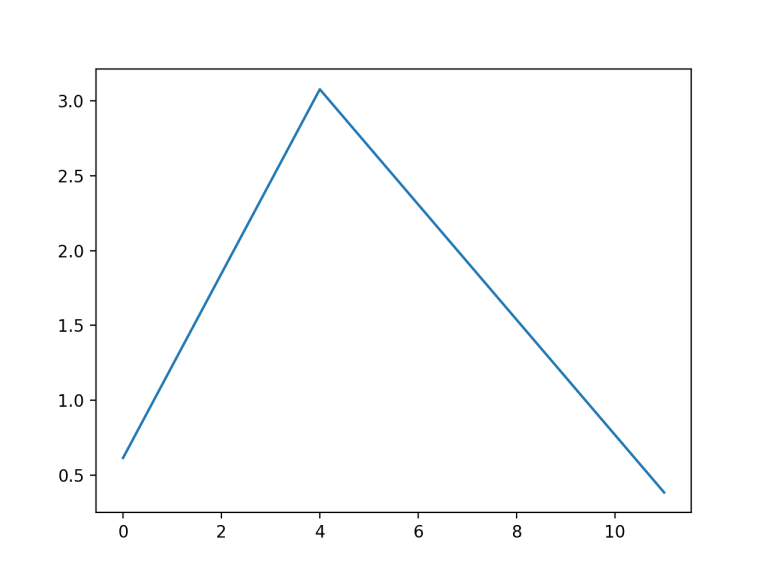
plt.plot(x)
plt.show()
Output:
tensor([ 0.,  0.,  0.,  0.,  0.,  0.,  0.,  0.,  0.,  0.,  0.,  0.])
None
tensor([ 2., -1., -1.,  2., -1., -1.,  2., -1., -1.,  2., -1.,  0.])
tensor([-1.,  2., -1., -1.,  2., -1., -1.,  2., -1., -1.,  2., -1.])
tensor([ 0., -1.,  2., -1., -1.,  2., -1., -1.,  2., -1., -1.,  2.])
tensor([[ 2., -1., -1.,  2., -1., -1.,  2., -1., -1.,  2., -1.,  0.],
        [-1.,  2., -1., -1.,  2., -1., -1.,  2., -1., -1.,  2., -1.],
        [ 0., -1.,  2., -1., -1.,  2., -1., -1.,  2., -1., -1.,  2.]])
[[ 2. -1. -1.  2. -1. -1.  2. -1. -1.  2. -1.  0.]
 [-1.  2. -1. -1.  2. -1. -1.  2. -1. -1.  2. -1.]
 [ 0. -1.  2. -1. -1.  2. -1. -1.  2. -1. -1.  2.]]
[[ 2.  2.  2.  2.  2.  2.  2.  2.  2.  2.  2.  2.]
 [-1. -1. -1. -1. -1. -1. -1. -1. -1. -1. -1.  0.]
 [ 0. -1. -1. -1. -1. -1. -1. -1. -1. -1. -1. -1.]]
[[ 2.  2.  2.  2.  2.  2.  2.  2.  2.  2.  2.  2.]
 [-1. -1. -1. -1. -1. -1. -1. -1. -1. -1. -1.  0.]]
[0.61538462 1.23076923 1.84615385 2.46153846 3.07692308 2.69230769
 2.30769231 1.92307692 1.53846154 1.15384615 0.76923077 0.38461538]
