Mixed Integer Programming & Quantization Error
I though of another fun use case of mixed integer programming the other day. The quantization part of a digital to analog converter is difficult to analyze by the techniques taught in a standard signals course (linear analysis, spectral techniques, convolution that sort of thing). The way it is usually done is via assuming the quantization error is a kind of randomized additive noise.
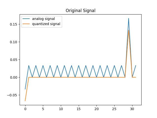
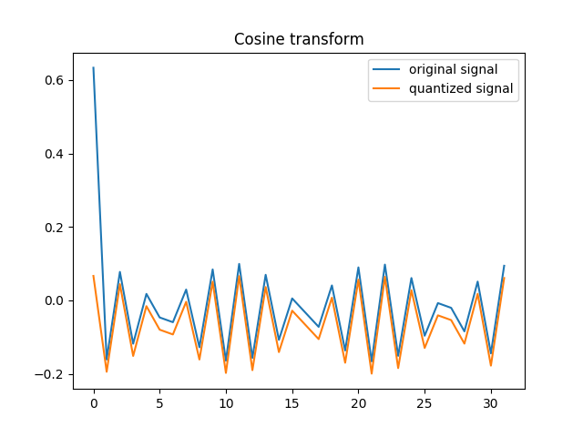
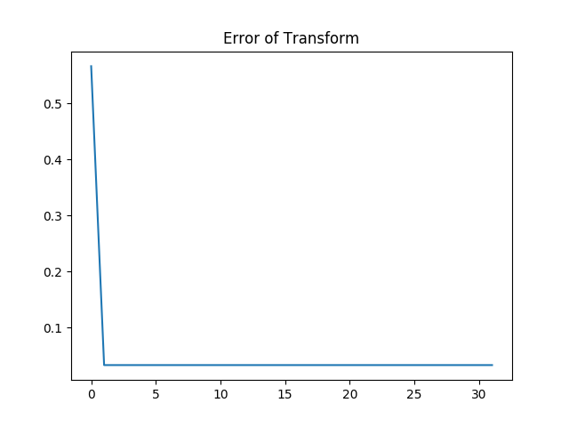
Mixed Integer programming does have the ability to directly encode some questions about this quantization though. We can directly encode the integer rounding relations by putting the constraint that the quantized signal is exactly +-1/2 a quantization interval away from the original signal. Then we can run further analysis on the signals and compare them. For example, I wrote down a quick cosine transform. Then I ask for the worst case signal that leads to the most error on the quantized transform versus the transform of the unquantized signal. My measure of worst case performance was the sum of the difference of the two transforms. I chose this because it is tractable as a mixed integer linear program. Not all reasonable metrics one might want will be easily encodable in a mixed integer framework it seems. Some of them are maximizing over a convex function, which is naughty. (for example trying to maximize the L2 error $ \sum|x-y|^2$ )
In a variant of this, it is also possible to directly encode the digital signal process in terms of logic gate construction and compare that to the intended analog transform, although this will be a great deal more computational expensive.
import cvxpy as cvx
import numpy as np
import matplotlib.pyplot as plt
N = 32
d = 15
x = cvx.Variable(N)
z = cvx.Variable(N, integer=True)
y = z / d # quantized signal. ~31 values between -1 and 1

constraints = []
constraints += [-1 <= y,  y <= 1, -1 <= x, x <= 1]

# roudning constraint. z = round(127*x)
constraints += [-0.5 <= d*x - z, d*x - z <= 0.5]
# an oppurtnitu for the FFT technique of Vanderbei


n = np.kron(np.arange(N), np.arange(N)).reshape((N,N))
U = np.cos( np.pi * n / N)
kx = U @ x
ky = U @ y

#hmmmm. Yes. Unfrotunately  I am asking a hard question?
# finding the minimum distortion signal is easy. finding the maximum distortion appears to be hard.
#This is not a convex objective : objective = cvx.Maximize(cvx.sum_squares(kx - ky))
# however, the following linearization does give us a maximally bad signal in a sense.
objective = cvx.Maximize(cvx.sum(kx - ky))

prob = cvx.Problem(objective, constraints)
prob.solve()
print(x.value)
plt.title("Original Signal")
plt.plot(x.value, label="analog signal")
plt.plot(y.value, label="quantized signal")
plt.figure()
plt.title("Error of Transform")
plt.plot(kx.value - ky.value)
plt.figure()
plt.title("Cosine transform")
plt.plot(kx.value, label="original signal")
plt.plot(ky.value, label="quantized signal")
plt.show()


This is interesting as a relatively straightforward technique for the analysis of quantization errors.
This also might be an interesting place to use the techniques of Vanderbei https://vanderbei.princeton.edu/tex/ffOpt/ffOptMPCrev4.pdf . He does a neato trick where he partially embeds the FFT algorithm into an optimization problem by adding auxiliary variables. Despite the expense of adding these variables, it greatly increases the sparsity of the constraint matrices, which will probably be a win. I wonder if one might do something similar with a Fast Multipole Method , Barnes Hut, or Wavelet transform? Seems likely. Would be neat, although I’m not sure what for. I was thinking of simulating the coulomb gas. That seems like a natural choice. Oooh. I should do that.