OSQP and Sparsegrad: Fast Model Predictive Control in Python for an inverted pendulum
OSQP is a quadratic programming solver that seems to be designed for control problems. It has the ability to warm start, which should make it faster.
I heard about it in this Julia talk
https://www.youtube.com/watch?v=dmWQtI3DFFo&t;=499s
They have some really cool technology over there in Julia land.
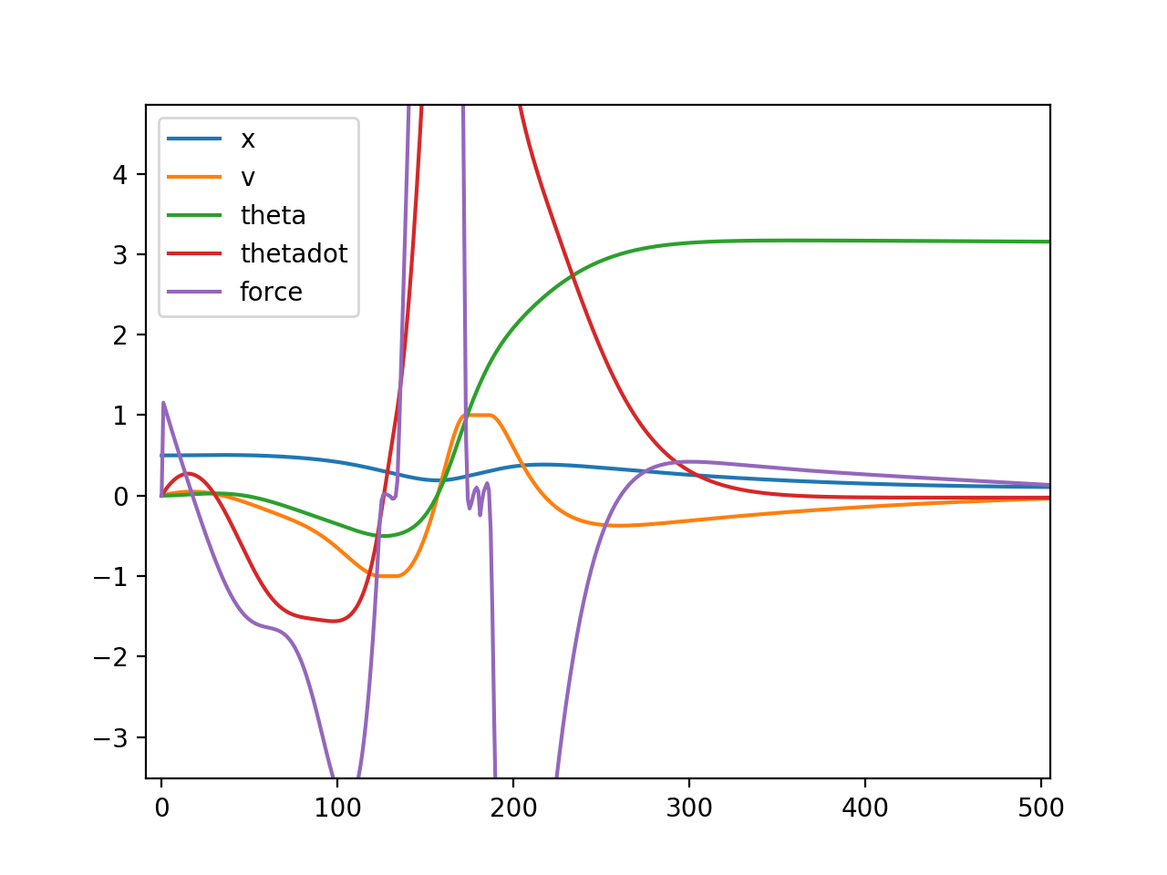
The problem is setup as a sequential quadratic program. I have a quadratic cost to try to bring the pendulum to an upright position.
The equations of motion are roughly
$ \ddot{\theta}I=-mgL\sin(\theta)+mfL\cos(\theta)$
$ \ddot{x}=f$
$ I=\frac{1}{3}mL^2$
We don’t include the back reaction of the pole on the cart. It is basically irrelevant for our systems and overly complicated for no reason. The interesting bit is the nonlinear dynamics and influence of the cart acceleration.
I write down obeying the equations of motion as a linear constraint between timesteps. I use sparsegrad to get a sparse Jacobian of the equations of motion. The upper and lower (l and u) bounds are set equal to make an equality constraint.
Our setup has a finite track about a meter long. Our motors basically are velocity control and they can go about +-1m/s. Both of these can be encapsulated as linear constraints on the position and velocity variables. $ l \le Ax \le u$
$ \phi(x)=0$
$ \phi(x) \approx \phi(x_0) + \partial \phi(x_0) (x - x_0)$
$ A= \partial \phi(x_0)$
$ l=u=\partial \phi(x_0) x_0 - \phi_0(x_0)$
Similarly for finding the quadratic cost function in terms of the setpoint $ x_s$. $ \frac{1}{2}x^T P x + q^Tx= \frac{1}{2}(x-x_s)P(x-x_s)$ Expanding this out we get
$ q = - Px_s$
I run for multiple iterations to hopefully converge to a solution (it does). The initial linearization might be quite poor, but it gets better.
The OSQP program seems to be able to run in under 1ms. Nice! Initial tests of our system seem to be running at about 100Hz.
Could probably find a way to make those A matrices faster than constructing them entirely anew every time. We’ll see if we need that.
I very inelegantly smash all the variables into x. OSQP and scipy sparse don’t support multiIndex objects well, best as I can figure. Vectors should be single dimensioned and matrices 2 dimensioned.
Still to be seen if it works on hardware. I was already having infeasibility problems. Adjusting the regularization on P seemed to help.
import sparsegrad.forward as forward
import numpy as np
import osqp
import scipy.sparse as sparse
import matplotlib.pyplot as plt
import time

#def f(x):
#	return x**2

#ad.test()
#print(dir(ad))
N = 1000
NVars  = 5
T = 5.0
dt = T/N
dtinv = 1./dt
#Px = sparse.eye(N)
#sparse.csc_matrix((N, N))
# The three deifferent weigthing matrices for x, v, and external force
reg = sparse.eye(N)*0.01
# sparse.diags(np.arange(N)/N)
P = sparse.block_diag([reg,reg ,sparse.eye(N), 1*reg,1*reg])
#P[N,N]=10
THETA = 2
q = np.zeros((NVars, N))
q[THETA,:] = np.pi
#q[N,0] = -2 * 0.5 * 10
q = q.flatten()
q= -P@q
#u = np.arr

x = np.random.randn(N,NVars).flatten()
#x = np.zeros((N,NVars)).flatten()
#v = np.zeros(N)
#f = np.zeros(N)


#print(f(ad.seed(x)).dvalue)


g = 9.8
L = 0.5
gL = g * L
m = 1.0 # doesn't matter
I = L**2 / 3
Iinv = 1.0/I
print(Iinv)


def constraint(var, x0, v0, th0, thd0):
	#x[0] -= 1
	#print(x[0])
	x = var[:N]
	v = var[N:2*N]
	theta = var[2*N:3*N]
	thetadot = var[3*N:4*N]
	a = var[4*N:5*N]
	dynvars = (x,v,theta,thetadot)
	xavg, vavg, thetavg, thdotavg = map(lambda z: (z[0:-1]+z[1:])/2, dynvars)
	dx, dv, dthet, dthdot = map(lambda z: (z[1:]-z[0:-1])*dtinv, dynvars)
	vres = dv - a[1:]
	xres = dx - vavg
	torque = -gL*np.sin(thetavg) + a[1:]*L*np.cos(thetavg)
	thetdotres = dthdot - torque*Iinv
	thetres = dthet - thdotavg

	return x[0:1]-x0, v[0:1]-v0, theta[0:1]-th0, thetadot[0:1]-thd0, xres,vres, thetdotres, thetres
	#return x[0:5] - 0.5


def getAlu(x, x0, v0, th0, thd0):
	gt = np.zeros((2,N))
	gt[0,:] = 0.1 # x is greaer than 0
	gt[1,:] = -1 #veclotu is gt -1m/s
	gt = gt.flatten()
	lt = np.zeros((2,N))
	lt[0,:] = 0.8
	lt[1,:] = 1 # velocity less than 1m/s
	lt = lt.flatten()

	z = sparse.bsr_matrix((N, N))
	ineqA = sparse.bmat([[sparse.eye(N),z,z,z,z],[z,sparse.eye(N),z,z,z]]) #.tocsc()
	print(ineqA.shape)
	#print(ineqA)
	cons = constraint(forward.seed_sparse_gradient(x), x0, v0, th0, thd0)
	A = sparse.vstack(map(lambda z: z.dvalue, cons)) #  y.dvalue.tocsc()
	print(A.shape)
	totval = np.concatenate(tuple(map(lambda z: z.value, cons)))
	temp = A@x - totval


	A = sparse.vstack((A,ineqA)).tocsc()

	#print(tuple(map(lambda z: z.value, cons)))
	print(temp.shape)
	print(lt.shape)
	print(gt.shape)
	u = np.concatenate((temp, lt))
	l = np.concatenate((temp, gt))
	return A, l, u


#A = y.dvalue.tocsc()
#print(y.dvalue)
#sparse.hstack( , format="csc")
A, l, u = getAlu(x, 0.5, 0, 0, 0)
m = osqp.OSQP()
m.setup(P=P, q=q, A=A, l=l, u=u) #  **settings
results = m.solve()
print(results.x)


#plt.plot(results.x[3*N:4*N])
#plt.plot(results.x[4*N:5*N])
start = time.time()
iters = 100
for i in range(iters):
	A, l, u = getAlu(results.x, 0.5, 0, 0, 0)
	print(A.shape)
	#print(len(A))
	m.update(Ax=A.data, l=l, u=u)
	results = m.solve()
end = time.time()
print("Solve in :", iters / (end-start) ,"Hz")

plt.plot(results.x[:N], label="x")
plt.plot(results.x[N:2*N], label="v")
plt.plot(results.x[2*N:3*N], label="theta")
plt.plot(results.x[3*N:4*N], label="thetadot")
plt.plot(results.x[4*N:5*N], label="force")
plt.legend()
plt.show()
#m.update(q=q_new, l=l_new, u=u_new)
