Performing Some Laplace Experiments
So I’m looking at the sparse solver capabilities of python.
Trying a 3d poisson problem (electrostatics of a point charge) in V=0 boundary conditions
$ \nabla^2 \phi = \delta^3 (x) $
from scipy import sparse
from scipy.sparse import linalg as la
import numpy as np


N = 25
L = 1.
dx = L/N
dx2 = dx**2
K1 = sparse.diags([1./dx2, -2/dx2, 1/dx2], [-1, 0, 1], shape=(N, N))
I = sparse.identity(N, format='dia')
K2 = sparse.kron(K1,I)+sparse.kron(I,K1)
I2 = sparse.kron(I,I)
K3 = sparse.kron(I,K2) + sparse.kron(K1,I2)

row  = np.array([N/2])
col  = np.array([0])
data = np.array([1/dx])
delta = sparse.coo_matrix((data, (row, col)), shape=(N,1)).tocsr()

source2 = sparse.kron(delta,delta)
source3 = sparse.kron(delta,source2)


phi = la.spsolve(K3, source3)
phi = phi.reshape((N,N,N))


x = np.linspace(0,L,N,endpoint=False)
y = np.linspace(0,L,N,endpoint=False)
z = np.linspace(0,L,N,endpoint=False)
xv, yv, zv = np.meshgrid(x,y,z)


# http://scikit-image.org/docs/dev/auto_examples/plot_marching_cubes.html
from skimage import measure
verts, faces = measure.marching_cubes(phi, -.1)
#print verts
verts = verts * L / N # rescale verts
from mpl_toolkits.mplot3d.art3d import Poly3DCollection


import matplotlib.pyplot as plt
from mpl_toolkits.mplot3d import Axes3D
fig = plt.figure()

ax = fig.add_subplot(111, projection='3d')
mesh = Poly3DCollection(verts[faces])
ax.add_collection3d(mesh)

#ax.set_xlim(0, 24)  # a = 6 (times two for 2nd ellipsoid)
#ax.set_ylim(0, 20)  # b = 10
#ax.set_zlim(0, 32)

plt.show()
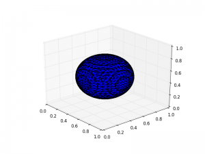
Looks like a sphere. Cool.
Using scikit-image for finding the isosurface (constant potential surface). Ripped right from their examples.
http://scikit-image.org/docs/dev/auto_examples/plot_marching_cubes.html
Note that it needs to be rescaled, since verts is in the integer index format.
Seems to work. Takes a couple seconds to finish on my macbook pro at N=25.
