Pytorch Trajectory Optimization 3: Plugging in the Hessian
I plugged in the hessian extraction code for using newton steps.
When I profiled it using the oh so convenient https://github.com/rkern/line_profiler I found almost all of my time was spent in the delLy.backwards step. For each hessian I needed to run this B (the band width) times and each time cost ~0.6ms. For the entire run to converge took about 70 iterations and 1000 runs of this backwards step, which came out to 0.6 seconds. It is insane, but actually even calculating the band of the hessian costs considerably more time than inverting it.
So to speed this up, I did a bizarre thing. I replicated the entire system B times. Then I can get the entire hessian band in a single call to backwards. remarkably, although B ~ 15 this only slowed backwards down by 3x. This is huge savings actually, while obviously inefficient. The entire program has gone down from 1.1s to 0.38s, roughly a 3x improvement. All in all, this puts us at 70/0.38 ~ 185 Hz for a newton step. Is that good enough? I could trim some more fat. The Fast MPC paper http://web.stanford.edu/~boyd/papers/fast_mpc.html says we need about ~5 iterations to tune up a solution, this would mean running at 40Hz. I think that might be ok.
Since the hessian is hermitian it is possible to use roughly half the calls (~B/2), but then actually extracting the hessian is not so simple. I haven’t figured out a way to comfortably do such a thing yet. I think I could figure out the first column and then subtract (roughly some kind of gaussian elimination procedure).
It has helped stability to regularize everything with a surprising amount of weight in the cost. I guess since I anticipate all values being in the range of -10,10, maybe this makes sense.
Now I need to try not using this augmented Lagrangian method and just switching to a straight newton step.
Edit: Ooh. Adding a simple backtracking line search really improves stability.
import torch
import matplotlib.pyplot as plt
import numpy as np
import torch.optim
from scipy import linalg

N = 100
T = 10.0
dt = T/N
NVars = 4
NControls = 1
batch = (NVars+NControls)*3
def getNewState():
 #we 're going to also pack f into here
 x = torch.zeros(batch,N,NVars+NControls, requires_grad=True)

 #f = torch.zeros(batch, N-1, requires_grad=True)

 l = torch.zeros(batch, N-1,NVars, requires_grad=False)
 return x, l

def calc_loss(x, l , rho, prox=0): # l,
 #depack f, it has one less time point
 cost = 0.1*torch.sum(x**2)
 #cost += prox * torch.sum((x - x.detach())**2)
 f = x[:,1:,:NControls]
 #leftoverf = x[:,0,:NControls]
 x = x[:,:,NControls:]

 delx = (x[:,1:,:] - x[:, :-1,:]) / dt

 xbar = (x[:,1:,:] + x[:, :-1,:]) / 2
 dxdt = torch.zeros(batch, N-1,NVars)
 THETA = 2
 THETADOT = 3
 X = 0
 V = 1
 dxdt[:,:,X] = xbar[:,:,V]
 #print(dxdt.shape)
 #print(f.shape)
 dxdt[:,:,V] = f[:,:,0]
 dxdt[:,:,THETA] = xbar[:,:,THETADOT]
 dxdt[:,:,THETADOT] = -torch.sin(xbar[:,:,THETA]) + f[:,:,0]*torch.cos(xbar[:,:,THETA])


 xres = delx - dxdt

 lagrange_mult = torch.sum(l * xres)


 #cost = torch.sum((x+1)**2+(x+1)**2, dim=0).sum(0).sum(0)
 #cost += torch.sum((f+1)**2, dim=0).sum(0).sum(0)
 #cost += 1
 penalty = rho*torch.sum( xres**2)


 #cost += 1.0*torch.sum((abs(x[:,:,THETA]-np.pi)), dim=1)
 #cost = 1.0*torch.sum((x[:,:,:]-np.pi)**2 )
 cost += 1.0*torch.sum((x[:,:,THETA]-np.pi)**2 * torch.arange(N) / N )
 cost += 0.5*torch.sum(f**2)
 #cost = 1.0*torch.sum((x[:,:,:]-np.pi)**2 )
 #cost = cost1 + 1.0
 #cost += 0.01*torch.sum(x**2, dim=1).sum(0).sum(0)
 #xlim = 3
 #cost += 0.1*torch.sum(-torch.log(xbar[:,:,X] + xlim) - torch.log(xlim - xbar[:,:,X]))
 #cost += 0.1*torch.sum(-torch.log(xbar[:,:,V] + 1) - torch.log(1 - xbar[:,:,V]),dim=1)
 #cost += (leftoverf**2).sum()


 #total_cost = cost + lagrange_mult + penalty

 return cost, penalty, lagrange_mult, xres

def getFullHess(): #for experimentation
 pass

def getGradHessBand(loss, B, x):
 #B = bandn
 delL0, = torch.autograd.grad(loss, x, create_graph=True)
 delL = delL0[:,1:,:].view(B,-1) #remove x0
 print("del ", delL[:,:10])
 #hess = torch.zeros(B,N-1,NVars+NControls, requires_grad=False).view(B,B,-1)
 y = torch.zeros(B,N-1,NVars+NControls, requires_grad=False).view(B,-1)

 #y = torch.eye(B).view(B,1,B)
 #print(y.shape)
 for i in range(B):
 #y = torch.zeros(N-1,NVars+NControls, requires_grad=False).view(-1)
 y[i,i::B]=1
 #print(y[:,:2*B])
 print(y.shape)
 print(delL.shape)
 delLy = torch.sum(delL * y)
 #print(delLy)


 delLy.backward() #(i != B-1)
 #torch.autograd.grad(loss, x, create_graph=True)
 #print(hess.shape)
 #print(x.grad.shape)
 #hess[i,:] = x.grad[:,1:,:].view(-1) #also remove x0
 #print(hess[i,:])
 #print(x.grad)

 #print(hess)
 nphess = x.grad[:,1:,:].view(B,-1).detach().numpy()# .view(-1)# hess.detach().numpy()
 #print(nphess[:,:4])
 #print(nphess)
 for i in range(B):
 nphess[:,i::B] = np.roll(nphess[:,i::B], -i+B//2, axis=0)
 print(nphess[:,:4])
 #hessband = removeX0(nphess[:B//2+1,:])
 #grad = removeX0(delL.detach().numpy())
 return delL.detach().numpy()[0,:], nphess #hessband

x, l = getNewState()
rho = 0.1
prox = 0.0
for j in range(10):
 while True:
 try:
 cost, penalty, lagrange_mult, xres = calc_loss(x, l, rho, prox)
 #print(total_cost)
 print("hey now")
 #print(cost)
 total_cost = cost + lagrange_mult + penalty
 #total_cost = cost
 gradL, hess = getGradHessBand(total_cost, (NVars+NControls)*3, x)
 #print(hess)
 #print(hess.shape)
 gradL = gradL.reshape(-1)
 #print(gradL.shape)

 #easiest thing might be to put lagrange mutlipleirs into x.
 #Alternatively, use second order step in penalty method.
 bandn = (NVars+NControls)*3//2
 print(hess.shape)
 print(gradL.shape)
 dx = linalg.solve_banded((bandn,bandn), hess, gradL) #
 x.grad.data.zero_()
 #print(hess)
 #print(hess[bandn:,:])
 #dx = linalg.solveh_banded(hess[:bandn+1,:], gradL, overwrite_ab=True)
 newton_dec = np.dot(dx,gradL)
 #df0 = dx[:NControls].reshape(-1,NControls)
 dx = dx.reshape(1,N-1,NVars+NControls)

 with torch.no_grad():
 x[:,1:,:] -= torch.tensor(dx)
 print(x[:,:5,:])
 #print(x[:,0,NVars:].shape)
 #print(df0.shape)
 costval = cost.detach().numpy()
 #break
 if newton_dec < 1e-10*costval:
 break
 except np.linalg.LinAlgError:
 print("LINALGERROR")
 prox += 0.1
 #break
 #print(x)
 with torch.no_grad():
 l += 2 * rho * xres
 rho = rho * 2 #+ 0.1
#print(x)
#plt.subplot(131)
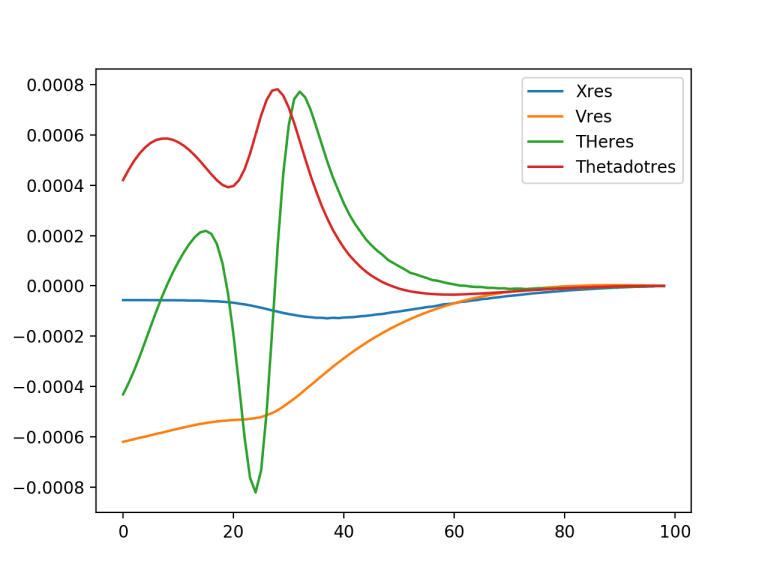
plt.plot(xres[0,:,0].detach().numpy(), label='Xres')
plt.plot(xres[0,:,1].detach().numpy(), label='Vres')
plt.plot(xres[0,:,2].detach().numpy(), label='THeres')
plt.plot(xres[0,:,3].detach().numpy(), label='Thetadotres')

plt.legend(loc='upper right')
plt.figure()
#plt.subplot(132)
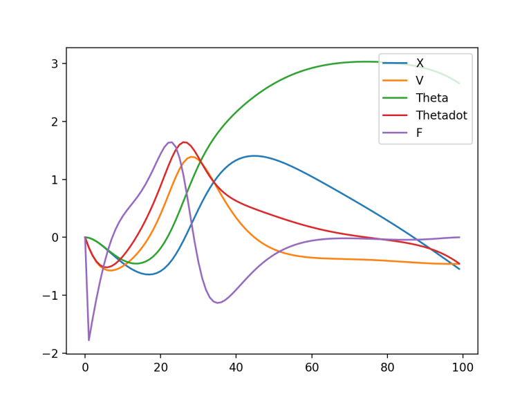
plt.plot(x[0,:,1].detach().numpy(), label='X')
plt.plot(x[0,:,2].detach().numpy(), label='V')
plt.plot(x[0,:,3].detach().numpy(), label='Theta')
plt.plot(x[0,:,4].detach().numpy(), label='Thetadot')
plt.plot(x[0,:,0].detach().numpy(), label='F')
#plt.plot(cost[0,:].detach().numpy(), label='F')
plt.legend(loc='upper right')
#plt.figure()
#plt.subplot(133)
#plt.plot(costs)


plt.show()

