Ray Tracing Algebraic Surfaces
Ray tracing is a natural way of producing computer images. One takes a geometrical ray that connects the pinhole of the camera to a pixel of the camera and find where it hits objects in the scene. You then color the pixel the color of the object it hit.
You can add a great deal of complexity to this by more sophisticated sampling and lighting, multiple bounces, strange surfaces, but that’s it in a nutshell.
A very popular tutorial on this is Ray Tracing in One Weekend https://raytracing.github.io/
There are a couple ways to do the geometrical collision detection part. One is to consider simple shapes like triangles and spheres and find closed form algorithms for the collision point. This is a fast and simple approach and the rough basis of the standard graphics pipeline. Another is to describe shapes via signed distance functions that tell you how far from the object you are and use ray-marching, which is a variant of newton’s method iteratively finding a position on a surface along the ray. ShaderToys very often use this technique.
If you describe your objects using algebraic (polynomial) equations, like $ x^2 + y^2 + z^2 - 1$ describes a sphere, there is the possibility of using root finding algorithms, which are readily available. I thought this was kind of neat. Basically the ray hitting the concrete pixel $ (x_0, y_0)$ can be parameterized by a univariate polynomial $ (x,y,z) = (\lambda x_0, \lambda y_0, \lambda)$ , which can be plugged into the multivariate polynomial $ (\lambda x_0)^2 + (\lambda y_0)^2 + \lambda^2 - 1$. This is a univariate polynomial which can be solved for all possible collision points via root finding. We filter for the collisions that are closest and in front of the camera. We can also use partial differentiation of the surface equations to find normal vectors at that point for the purposes of simple directional lighting.
As is, it really isn’t very fast but it’s short and it works.
Three key packages are
- https://github.com/JuliaAlgebra/TypedPolynomials.jl for multivariate polynomials
- https://juliamath.github.io/Polynomials.jl/stable/ for univariate polynomials
- https://github.com/JuliaImages/Images.jl Images for drawing Images
using Images
using LinearAlgebra
using TypedPolynomials
using Polynomials

function raytrace(x2,y2,p)
    z = Polynomials.Polynomial([0,1])

    # The ray parameterized by z through the origin and the point [x2,y2,1]
    x3 = [z*x2, z*y2, z]

    # get all the roots after substitution into the surface equation
    r = roots(p(x=>x3))


    # filter to use values of z that are real and in front of the camera
    hits = map(real, filter( x -> isreal(x) & (real(x) > 0.0)  , r))

    if length(hits) > 0
        l = minimum(hits) # closest hit only
        x3 = [z(l) for z in x3]
        # get normal vector of surface at that point
        dp = differentiate(p, x)
        normal = normalize([ z(x=> x3)  for z in dp])
        # a little directional and ambient shading
        return max(0,0.5*dot(normal,normalize([0,1,-1]))) + 0.2
    else
        return 0 # Ray did not hit surface
    end
end

@polyvar x[1:3]

# a sphere of radius 1 with center at (0,0,3)
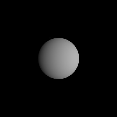
p = x[1]^2 + x[2]^2 + (x[3] - 3)^2 - 1

box = -1:0.01:1
Gray.([ raytrace(x,y,p) for x=box, y=box ])

Sphere.
@polyvar x[1:3]
R = 2
r = 1

# another way of doing offset
x1 = x .+ [ 0, 0 , -5 ]

# a torus at (0,0,5)
# equation from https://en.wikipedia.org/wiki/Torus
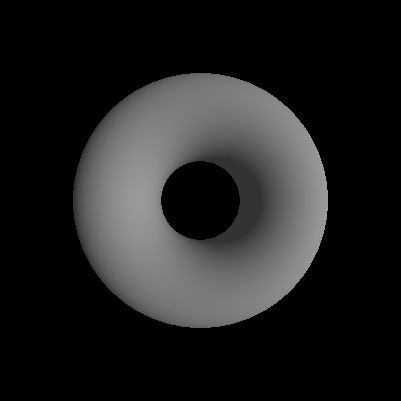
p = (x1[1]^2 + x1[2]^2 + x1[3]^2 + R^2 - r^2)^2 - 4R^2 * (x1[1]^2 + x1[2]^2)

box = -1:0.005:1
img = Gray.([ raytrace(x,y,p) for x=box, y=box ])
save("torus.jpg",img)
 Torus
Torus
Some thoughts on speeding up: Move polynomial manipulations out of the loop. Perhaps partial evaluate with respect to the polynomial? That’d be neat. And of course, parallelize