Answer Set Programming for E-Graph DAG Extraction
E-graphs (equivalence graphs) are a data structures for efficiently and compactly storing many equivalent versions of expressions. They are useful for performing compiler optimizations and theorem proving.
Ultimately, one is interested in extracting out a version of an expression from inside the egraph with good properties so you can turn it into efficient code or a piece of hardware. This problem can be hard depending on how you want to model it.
Answer Set Programming is a paradigm for solving combinatorial satisfaction or optimization problems. It offers some unusual well-foundedness/justification/supported-set modelling capabilities not offered by SAT, CSP, ILP, or SMT solvers. It is exactly this aspect that makes it very useful for a particular model of the extraction problem. The ASP solver clingo is roughly a datalog-like grounder gringo that feeds into a SAT-like solver clasp with intrinsic loop breaking constraints support. That Remy independently had this idea is encouraging that it is a good one, since he is often right.
Tree vs DAG Extraction
A method for certain cost models is to apply dynamic programming. In this model, the cost of a enode in the egraphs is a function of the minimal cost of its children. Very natural right? You can compute the best cost as a fixed point calculation, taking the best enode for each eclass to be the one who’s cost is currently smallest. This will converge fairly quickly.
It occurs rather often that this framework does not model the actual costs well, in particular in regards to sharing. Shared subexpressions can be reused cheaply. In this case, what one wants to extract is not an optimal AST, but instead an optimal DAG. The cost function of the DAG is intrinsically more nonlocal or noncompositional than the cost function of an AST. It may be desirable to pick a locally less optimal subexpression, if that subexpression has more reusable parts elsewhere.
A simple additive tree cost model is $\sum_n c_n m_n$ where $c_n$ is the cost of enode $n$ and $m_n$ is the multiplicity you have picked it.
The DAG cost model would instead be $\sum_n c_n b_n$ where instead $b_n$ is not a boolean 0-1 variable saying whether you picked the node or not.
In either case, the optimization problem is constrained to be selecting subgraphs of the egraph which form valid trees or valid DAGs. Tree-ness or DAG-ness is a subtle property that is surprisingly difficult/impossible to describe in first order logic. It is an example where you need a notion of least fixed point in your logic.
See for example:
This axiom expresses that if all of your children are valid trees, then you are a valid tree.
Tree(node) = (forall c, child(c,node) => Tree(c)).
This axiom is loose however to the notion of tree-ness. Tree(C) := true is a valid model of this axiom, that just says every node is a tree in any graph.
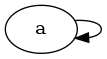
As a second counterexample, consider a graph with a single vertex a and a single self edge a -> a. Obviously this node is not a tree. But it is self consistent to say a is a tree node according to our bad definition, since indeed all of it’s children are also tree nodes.
Ok, you might try to patch this up by saying trees have no self loops but an extension of this counterexample is to consider a giant loop of arbitrarily large size N. How can you fight this?
What we want to express is that we can iteratively find the trees by first saying any leaf (no children) is a tree, then keep increasing our class of tree things to include anything with all children we have already determined to be trees. This is a very intuitive interpretation of a notion of implication =>, but it is not the classical first order logic notion.
It is exactly what datalog or answer set programming does though. It is :-. Note that until you start using non-stratified negation, answer set programming and datalog are essentially identical (ASP treats negation “presciently”/self-consistently. You check an ASP solution by running datalog on using current derived atoms for positive atoms but the guessed final solution for the negated atoms). They both allow you to derive a minimal model or least fixed point of a pile of horn clauses.
node(1..4).
edge((1,2);(2,3)).
edge((4,4)).


tree(N) :- node(N), tree(C) : edge((C,N)).

% Answer: 1
% node(1) node(2) node(3) node(4) edge((1,2)) edge((2,3)) tree(4) tree(1) tree(2) tree(3)
% SATISFIABLE
It is exactly this property that makes it possible to require to extract only the DAGs to the ASP solver in a very natural way.
Extraction Model
The ASP model starts with some description of a fixed egraph described as a pile of relations.
For example, an encoding of the egraph resulting from x + y = y + x might look like
% enode(eid, symbol, child_eid...)
enode(1,"add",2,3).
enode(1,"add",3,2).
enode(2, "x").
enode(3, "y").
However, it is convenient to not have to deal with different numbers of arguments separately, so instead I encode this using a enode identifier.
% enode(eid, enode_id, sym)
% child(eid, enode_id, child_eid)
enode(1,0,"add").
child(1,0,2).
child(1,0,3).

enode(1,1,"add").
child(1,0,3).
child(1,0,2).

enode(2,0,"x").
enode(3,0,"y").
In answer set programming, the notation { a } is how you represent the option to pick a to be true or false. We may only pick an enode if it’s children have been picked. This is the DAG property.
% We may choose to select this enode if we have selected that class of all its children.
{ sel(E,I) } :- enode(E,I,_,_), selclass(Ec) : child(E,I,Ec).
It is convenient for modelling to have an auxiliary predicate for selecting an eclass. We select an eclass if we select a node in the eclass.
% if we select an enode in an eclass, we select that eclass
selclass(E) :- sel(E,_).
We want to disallow any solution where we don’t select the root.
% It is inconsistent for a eclass to be a root and not selected.
:- root(E), not selclass(E).
This is subtly different from saying we pick the root, which I would write like so
% NO. WE DON'T WANT THIS
selclass(E) :- root(E).
These statements are classically equivalent , but they are not ASP equivalent. I can show the classical equivalence using the ASP invalid identity A => B == not A \/ B.
forall E, root(E) /\ not selclass(E) => false == not root(E) \/ not not selclass(E) \/ false == not root(E) \/ selclass(E) and forall E, root(E) => selclass(E) == not root(E) \/ selclass(E).
If we added this axiom, we’d allow picking a solution where we pick the root but do not require the root’s children to be picked first. This is again a subtle use of ASP modeling, but it’s exactly the subtly we want to express the required DAGness of the desired solution.
Finally, we want to minimize the cost of the selected enodes.
#minimize { C,E,I : sel(E,I), enode(E,I,_,C) }.
It seems to help the solve time to add that we don’t expect more than 1 enode to be select per eclass in the minimizing model.
% optional constraints to help?
:- enode(E,_,_,_), #count { E,I : sel(E,I)} > 1.
The short nature of the encoding reflects that ASP is a very natural framework for this problem. ASP has a number of different solver architectures, but a basic gist of some is that they are roughly SAT solvers + learned cycle breaking / support constraints. In most other solvers, these cycle breaking constraints must be eagerly produced (this is also done in the types of ASP solvers that eagerly compile to SAT).
Rust Encoding
Max has been starting to cook up an extraction gym. I don’t know that it is fully baked ready for contributors yet (although I think more benchmark egraphs are welcome).
I had to root around a bit in the rust bindings to figure out how to run clingo programmatically, but it’s not that bad. You build a solver, add facts and rules, call the grounder (roughly an over approximating datalog run), then the solver which returns a sequence of increasingly good solutions.
It appears to be slow on the large problems. There is probably still refinement / redundant constraints / symmettry breaking / hints that could speed it up. In addition, giving an upper bound cost from the bottom up method may speed it up.
I bet heuristic methods might be better in terms of solve time / solution quality tradeoff, but still this is quite nice.
use super::*;
use clingo::control;

use clingo::ClingoError;
use clingo::FactBase;
use clingo::ShowType;
use clingo::Symbol;
use clingo::ToSymbol;

// An enode is identified with the eclass id and then index in that eclasses enode list.
#[derive(ToSymbol)]
struct Enode {
    eid: u32,
    node_i: u32,
    op: String,
    cost: i32,
}

#[derive(ToSymbol)]
struct Root {
    eid: u32,
}

#[derive(ToSymbol)]
struct Child {
    eid: u32,
    node_i: u32,
    child_eid: u32,
}

const ASP_PROGRAM: &str = "
% we may choose to select this enode if we have selected that class of all it's children.
{ sel(E,I) } :- enode(E,I,_,_), selclass(Ec) : child(E,I,Ec).

% if we select an enode in an eclass, we select that eclass
selclass(E) :- sel(E,_).

% It is inconsistent for a eclass to be a root and not selected.
% This is *not* the same as saying  selclass(E) :- root(E).
:- root(E), not selclass(E).

:- enode(E,_,_,_), #count { E,I : sel(E,I)} > 1.

#minimize { C,E,I : sel(E,I), enode(E,I,_,C) }.

#show sel/2.
";

pub struct AspExtractor;
impl Extractor for AspExtractor {
    fn extract(&self, egraph: &SimpleEGraph, _roots: &[Id]) -> ExtractionResult {
        let mut ctl = control(vec![]).expect("REASON");
        // add a logic program to the base part
        ctl.add("base", &[], ASP_PROGRAM)
            .expect("Failed to add a logic program.");

        let mut fb = FactBase::new();
        for eid in egraph.roots.iter() {
            let root = Root {
                eid: (*eid).try_into().unwrap(),
            };
            fb.insert(&root);
        }
        for (_i, class) in egraph.classes.values().enumerate() {
            for (node_i, node) in class.nodes.iter().enumerate() {
                let enode = Enode {
                    eid: class.id.try_into().unwrap(),
                    node_i: node_i.try_into().unwrap(),
                    op: node.op.clone(),
                    cost: node.cost.round() as i32,
                };
                fb.insert(&enode);
                for child_eid in node.children.iter() {
                    let child = Child {
                        eid: class.id.try_into().unwrap(),
                        node_i: node_i.try_into().unwrap(),
                        child_eid: (*child_eid).try_into().unwrap(),
                    };
                    fb.insert(&child);
                }
            }
        }

        ctl.add_facts(&fb).expect("Failed to add factbase");
        let part = clingo::Part::new("base", vec![]).unwrap();
        let parts = vec![part];
        ctl.ground(&parts).expect("Failed to ground");
        let mut handle = ctl
            .solve(clingo::SolveMode::YIELD, &[]) // maybe use ctl.optimal_models()
            .expect("Failed to solve");
        let mut result = ExtractionResult::new(egraph.classes.len());
        while let Some(model) = handle.model().expect("model failed") {
            let atoms = model
                .symbols(ShowType::SHOWN)
                .expect("Failed to retrieve symbols in the model.");
            for symbol in atoms {
                assert!(symbol.name().unwrap() == "sel");
                let args = symbol.arguments().unwrap();
                result.choices[args[0].number().unwrap() as usize] =
                    args[1].number().unwrap() as usize;
            }

            handle.resume().expect("Failed resume on solve handle.");
        }
        handle.close().expect("Failed to close solve handle.");
        result
    }
}
Clingraph
A really cool and useful utility for working with clingo is clingraph. It let’s you visualize solutions directly out of clingo. It is actually a separate command that you can pipe other stuff into as well.
Here is a solution visualized out of the egg::test_fn! {math_powers, rules(), "(* (pow 2 x) (pow 2 y))" => "(pow 2 (+ x y))"} example.
It is slightly easier for me to draw the egraph as a bipartite graph between eclasses and enodes than the typical “eclass as dotted box surrounding enodes” visualization. Selected eclasses are colored red and selected enodes are colored cyan.
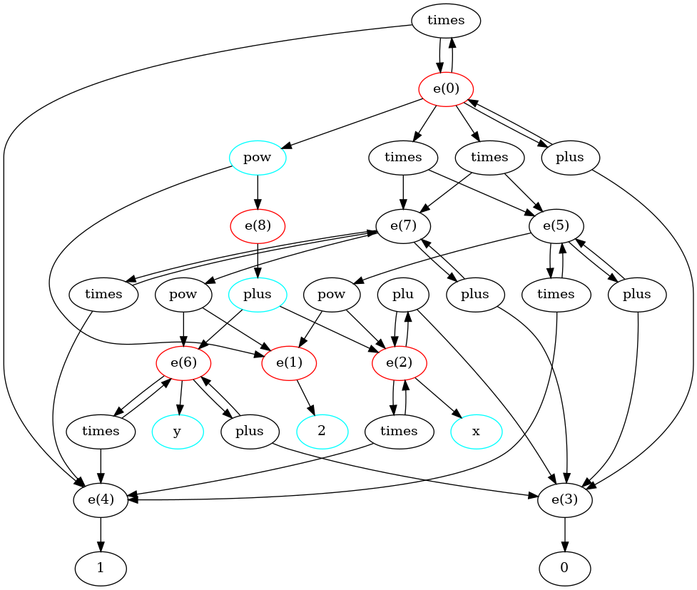
The example below is a bash script showing the clingraph invocation.
echo "
%re
root(0).
enode(0,0,"plus",1).
child(0,0,0).
child(0,0,3).
enode(0,1,"times",1).
child(0,1,5).
child(0,1,7).
enode(0,2,"times",1).
child(0,2,7).
child(0,2,5).
enode(0,3,"times",1).
child(0,3,0).
child(0,3,4).
enode(0,4,"pow",1).
child(0,4,1).
child(0,4,8).
enode(1,0,"2",1).
enode(2,0,"plu",1).
child(2,0,2).
child(2,0,3).
enode(2,1,"times",1).
child(2,1,2).
child(2,1,4).
enode(2,2,"x",1).
enode(3,0,"0",1).
enode(4,0,"1",1).
enode(5,0,"plus",1).
child(5,0,5).
child(5,0,3).
enode(5,1,"times",1).
child(5,1,5).
child(5,1,4).
enode(5,2,"pow",1).
child(5,2,1).
child(5,2,2).
enode(6,0,"plus",1).
child(6,0,6).
child(6,0,3).
enode(6,1,"times",1).
child(6,1,6).
child(6,1,4).
enode(6,2,"y",1).
enode(7,0,"plus",1).
child(7,0,7).
child(7,0,3).
enode(7,1,"times",1).
child(7,1,7).
child(7,1,4).
enode(7,2,"pow",1).
child(7,2,1).
child(7,2,6).
enode(8,0,"plus",1).
child(8,0,2).
child(8,0,6).

% we may choose to select this enode if we have selected that class of all it's children.
{ sel(E,I) } :- enode(E,I,_,_), selclass(Ec) : child(E,I,Ec).

% if we select an enode in an eclass, we select that eclass
selclass(E) :- sel(E,_).

% It is inconsistent for a eclass to be a root and not selected.
:- root(E), not selclass(E).

% This is *not* the same as saying  selclass(E) :- root(E).

%#minimize { 1,E : selclass(E) }.
#minimize { C,E,I : sel(E,I), enode(E,I,_,C) }.


% optional constrains to help?
:- enode(E,_,_,_), #count { E,I : sel(E,I)} > 1.


% GRAPHING STUFF

node((E,I)) :- enode(E,I,S,_).
%node((sym,S)) :- enode(E,I,S,_).
node(e(E)) :- enode(E,_,_,_).

edge(((E,I),e(Ec))) :- child(E,I,Ec).
edge((e(E),(E,I))) :- enode(E,I,_,_).
%edge(((E,I),(sym,S))) :- enode(E,I,S,_).

attr(node, (E,I), label, S) :- enode(E,I,S,_).

% visualize solution
attr(node, (E,I), color, cyan) :- sel(E,I).
attr(node, e(E), color, red) :- selclass(E).

%#show sel/2.
%#show selclass/1.


% analysis

%treecost(E,C1) :- enode(E,_,_,_), C1 = #min { C,E,I : treecost(E,I,C) }.
%treecost(E,I,C1 + Cs) :- enode(E,I,_,C1), Cs = #sum { C, Ec : child(E,I,Ec)}.

% :- #sum { C,E,I : sel(E,I), enode(E,I,_,C) } <= #sum { C,E : root(E), treecost(E,C)}.

% is this redundant or not?
% :- sel(E,I), child(E,I,Ec), { sel(Ec,I) : enode(Ec,I,_,_) } = 0.

" | clingo   \
--quiet=1 --outf=2 |  clingraph --view --out=render --format=png --dir=/tmp/clingraph --type=digraph
Blah Blah Blah
I could, and possibly should, label the children of an enode by their order, but it doesn’t matter
Ok, well we could add another axiom to tighten it up
Tree(node) = (forall c, child(c,node) => Tree(c)).
Leaf nodes with no children are Tree.
Transitive closure and first order logic
Why can’t reachability be expressed in first order logic?
If you try to express reachability, the system is free to overapproximate the notion of reachability.
echo "
node(a).
node(b).
edge((a,b)).
edge((b,b)).

dag(X) :- node(X), sel(Y) : edge((X,Y)).

% visualize solution
 attr(node, N, color, cyan) :- dag(N).

" | clingo --outf=2 |
    clingraph --view --out=render --format=png --dir=/tmp/clingraph --type=digraph
Weighting the selected edges is the analog of tree extraction
Examples
Blocking Cycles
f(f(f(a))) = f(f(a))
a(0).
f(0,1).
f(1,2).
f(2,3).
The aegraph may not have these problems. Another point in it’s favor.
Sharing
We want to notice sharing because sometimes it may be better
foo(large, large) = foo(large-1, large1-1) sharing breaking. Weird.
foo(bar(bar(x)), bar(bar(x))))) = foo(biz(x), baz(x))
Silly example:
x+y+z+x+y+w = 2*(x+y) + z + w Well, if we had that explicit rewrite that’d be cool. That turns sharing into explicit sharing.
So we need something that doesn’t have syntax? Or we want to avoid expensive “let” rules.
The tree selection problem
The canonical datalog program is the path program. This shows that datalog is capabble of expressing trasnitivty/ transitive closure
path(X,Y) :- edge(X,Y), path(Y,Z).
istree(X) :- node(X), not path(X,X).
Doesn’t make much sense unless we can have choice over children (like in egraph). So why even bother abstracting the problem?
Social network, pick a pyramid scheme. No loops, pick from your friends to maximize
echo "
node(a).
edge((a,a)).
" | clingo   \
--quiet=1 --outf=2 |  clingraph --view --out=render --format=png --dir=/tmp/clingraph --type=digraph
% DP cost treecost(E,C1) :- enode(E,,,), C1 = #min { C,E,I : treecost(E,I,C) }. treecost(E,I,C1 + Cs) :- enode(E,I,,C1), Cs = #sum { C, Ec : child(E,I,Ec)}.
% tree cost of actual selection overcost(E) overcost(E,I,C) :- sel(E,I), enode(E,I,_,C), #sum { C1, : selclass(Ec), child(), overcost(E,C1) }. ovrcost(E,C) :- overcost(E,I,C).
Hmm. but we can’t guarantee the tree cost of selection will be better. Can we count usages? Usages compound?
:- treecost(E,C), overcost().
% :- #sum { C,E,I : sel(E,I), enode(E,I,_,C) } <= #sum { C,E : root(E), treecost(E,C)}.
% is this redundant or not? % :- sel(E,I), child(E,I,Ec), { sel(Ec,I) : enode(Ec,I,,) } = 0.
```clingo
enode(0,0,"+",1).
child(0,0,1).
child(0,0,1). % hmm. deduplication
enode(1,0,a,1).
enode(1,1,b,2).

treecost(E,C1) :- enode(E,_,_,_), C1 = #min { C,I : treecost(E,I,C) }.
treecost(E,I,C1 + Cs) :- enode(E,I,_,C1), Cs = #sum { C, Ec : child(E,I,Ec), treecost(Ec,C)}.

:- #sum { C,E : root(E), treecost(E,C) } >

%unique(E) :- selclass(E), not selclass(E2), child(E1,I1,E), child(E2,I2,E), E1 != E2.
%-unique(E) :- selclass(E1), selclass(E2), child(E1,I1,E), child(E2,I2,E), E1 != E2.

% we count the number of selected parents
uses(E,U) :- enode(E,_,_,_), U = #count { Ep,I : sel(Ep,I), child(Ep,I,E)  }.

% tree cost of only uniquely owned. Could recursive call be treecost?
ucost(E,C) :- C = #sum { Cc,Ec : sel(E,I), child(E,I,Ec), uses(Ec,1), ucost(Ec,Cc) }.

% tempting for som reaosn. Charge each usage equally. But I don't think it can be dgnified
%ucost(E,C) :- C = #sum { Cc/U,Ec : sel(E,I), child(E,I,Ec), uses(Ec,U), ucost(Ec,Cc) }.

% if you have unique ownership, you
:- ucost(E,C) > treecost(E,C).
treecost(E,C1) :- eclass(E), C1 = #min { C,I : treecost(E,I,C) }.
treecost(E,I,C1 + Cs) :- enode(E,I,_,C1), Cs = #sum { C, Ec : child(E,I,Ec), treecost(Ec,C)}.

:- S1 = #sum { C,E : root(E), treecost(E,C) }, S2 = #sum { C,E,I : sel(E,I), enode(E,I,_,C) }, S1 > S2.
% tie breaking soft constraints?
% we count the number of selected parents
%uses(E,U) :- selclass(E), U = #count { Ep,I : sel(Ep,I), child(Ep,I,E) }.
%#maximize { U@0,E : uses(U,E) }. % we want to reuse eclasses

%#maximize { E@0,E : selclass(E) }.

%#minimize { E*I@0,E,I : sel(E,I) }.
#minimize { I@1,E,I : sel(E,I) }. % symmetry break to just prefer lower I?

%#minimize { 1@2,E : selclass(E) }. % minimizing number of eclasses is a decent heuristic

%:~ sel(E,I) [I@1]

%#heuristic selclass(E). [1@1, false]
%#heuristic sel(E,I). [2@2, false]

%:- S = #sum { C,E,I : sel(E,I), enode(E,I,_,C) }, S > 14.

treecost(E,C1) :- eclass(E), C1 = #min { C,E,I : treecost(E,I,C) }.
treecost(E,I,C1 + Cs) :- enode(E,I,_,C1), Cs = #sum { C, Ec : child(E,I,Ec), treecost(Ec,C) }, Cs < 15.
treesel(E,I) :- treecost(E,I,C), treecost(E,C).
%#maximize { 1/C@2,E,I : treecost(E,I,C), sel(E,I)}.

#maximize { 1@2,E : treesel(E,I), sel(E,I)}.

%#maximize { 1@2,E,I : sel(E,I), bottomsel(E,I)}.


% The idea here is maybe the local tree cost is a useful guide.
%estcost(E,C) :- estcost(E,I,C).
%estcost(E,I,C1 + Cs) :- sel(E,I), enode(E,I,_,C1), Cs = #sum { C, Ec : child(E,I,Ec), estcost(Ec,C)}, Cs < 10.
%#minimize { C@2,E,I : estcost(E,I,C)}.


%rootcost(S1) :-  S1 = #sum { C,E : root(E), treecost(E,C) }.
%:- rootcost(S1), S2 = #sum { C,E,I : sel(E,I), enode(E,I,_,C) }, S1 > S2.


% tree cost of only uniquely owned. Could recursive call be treecost?
%ucost(E,C) :- ucost(E,I,C).
%ucost(E,I,C1 + Cs) :- enode(E,I,_,C1), sel(E,I),  Cs = #sum { C, Ec : child(E,I,Ec), uses(Ec, 1), ucost(Ec,C)}, Cs < 40.

% if you have unique ownership, you
%:- selclass(E), ucost(E,C1), treecost(E,C), C1 > C.